Evaluating real-time performance#
Introduction#
Autoware should be real-time system when integrated to a service. Therefore, the response time of each callback should be as small as possible. If Autoware appears to be slow, it is imperative to conduct performance measurements and implement improvements based on the analysis. However, Autoware is a complex software system comprising numerous ROS 2 nodes, potentially complicating the process of identifying bottlenecks. To address this challenge, we will discuss methods for conducting detailed performance measurements for Autoware and provide case studies. It is worth noting that multiple factors can contribute to poor performance, such as scheduling and memory allocation in the OS layer, but our focus in this page will be on user code bottlenecks. The outline of this section is as follows:
- Performance measurement
- Single node execution
- Prepare separated cores
- Run single node separately
- Measurement and visualization
- Case studies
- Sensing component
- Planning component
Performance measurement#
Improvement is impossible without precise measurements. To measure the performance of the application code, it is essential to eliminate any external influences. Such influences include interference from the operating system and CPU frequency fluctuations. Scheduling effects also occur when core resources are shared by multiple threads. This section outlines a technique for accurately measuring the performance of the application code for a specific node. Though this section only discusses the case of Linux on Intel CPUs, similar considerations should be made in other environments.
Single node execution#
To eliminate the influence of scheduling, the node being measured should operate independently, using the same logic as when the entire Autoware system is running.
To accomplish this, record all input topics of the node to be measured while the whole Autoware system is running.
To achieve this objective, a tool called ros2_single_node_replayer has been prepared.
Details on how to use the tool can be found in the README.
This tool records the input topics of a specific node during the entire Autoware operation and replays it in a single node with the same logic.
The tool relies on the ros2 bag record command, and the recording of service/action is not supported as of ROS 2 Humble, so nodes that use service/action as their main logic may not work well.
Prepare separated cores#
Isolated cores running the node to be measured must meet the following conditions.
- Fix CPU frequency and disable turbo boost
- Minimize timer interruptions
- Offload RCU (Read Copy Update) callback
- Isolate the paired core if hyper-threading enabled
To fulfill these conditions on Linux, a custom kernel build with the following kernel configurations is required. You can find many resources to instruct you on how to build a custom Linux kernel (like this one). Note that even if full tickless is enabled, timer interrupts are generated for scheduling if more than two tasks exist in one core.
# Enable CONFIG_NO_HZ_FULL
-> General setup
-> Timers subsystem
-> Timer tick handling (Full dynticks system (tickless))
(X) Full dynticks system (tickless)

# Allows RCU callback processing to be offloaded from selected CPUs
# (CONFIG_RCU_NOCB_CPU=y)
-> General setup
-> RCU Subsystem
-*- Offload RCU callback processing from boot-selected CPUs
Additionally, the kernel boot parameters need to be set as follows.
GRUB_CMDLINE_LINUX_DEFAULT=
  "... isolcpus=2,8 rcu_nocbs=2,8 rcu_nocb_poll nohz_full=2,8 intel_pstate=disable”
In the above configuration, for example, the node to be measured is assumed to run on core 2, and core 8, which is a hyper-threading pair, is also being isolated.
Appropriate decisions on which cores to run the measurement target and which nodes to isolate need to be made based on the cache and core layout of the measurement machine.
You can easily check if it is properly configured by running cat /proc/softirqs.
Since intel_pstate=disable is specified in the kernel boot parameter, userspace can be specified in the scaling governor.
cat /sys/devices/system/cpu/cpu2/cpufreq/scaling_governor // ondemand
sudo sh -c "echo userspace > /sys/devices/system/cpu/cpu2/cpufreq/scaling_governor"
This allows you to freely set the desired frequency within a defined range.
sudo sh -c "echo <freq(kz)> > /sys/devices/system/cpu/cpu2/cpufreq/scaling_setspeed"
Turbo Boost needs to be switched off on Intel CPUs, which is often overlooked.
sudo sh -c "echo 0 > /sys/devices/system/cpu/cpufreq/boost"
Run single node separately#
Following the instructions in the ros2_single_node_replayer README, start the node and play the dedicated rosbag created by the tool.
Before playing the rosbag, appropriately set the CPU affinity of the thread on which the node runs, so it is placed on the isolated core prepared.
taskset --cpu-list -p <target cpu> <pid>
To avoid interference in the last level cache, minimize the number of other applications running during the measurement.
Measurement and visualization#
To visualize the performance of the measurement target, embed code for logging timestamps and performance counter values in the target source code.
To achieve this objective, a tool called pmu_analyzer has been prepared.
Details on how to use the tool can be found in the README. This tool can measure the turnaround time of any section in the source code, as well as various performance counters.
Case studies#
In this section, we will present several case studies that demonstrate the performance improvements. These examples not only showcase our commitment to enhancing the system's efficiency but also serve as a valuable resource for developers who may face similar challenges in their own projects. The performance improvements discussed here span various components of the Autoware system, including sensing modules and planning modules. There are tendencies for each component regarding which points are becoming bottlenecks. By examining the methods, techniques, and tools employed in these case studies, readers can gain a better understanding of the practical aspects of optimizing complex software systems like Autoware.
Sensing component#
First, we will explain the procedure for performance improvement, taking the node ring_outlier_filter as an example.
Refer to the Pull Request for details.
The following figure is a time-series plot of the turnaround time of the main processing part of ring_outlier_filter, analyzed as described in the "Performance Measurement" section above.
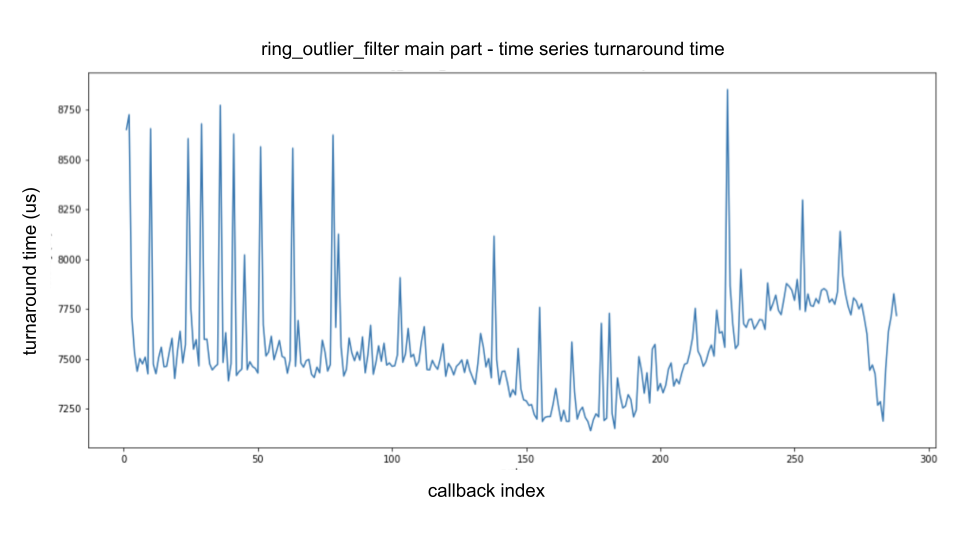
The horizontal axis indicates the number of callbacks called (i.e., callback index), and the vertical axis indicates the turnaround time.
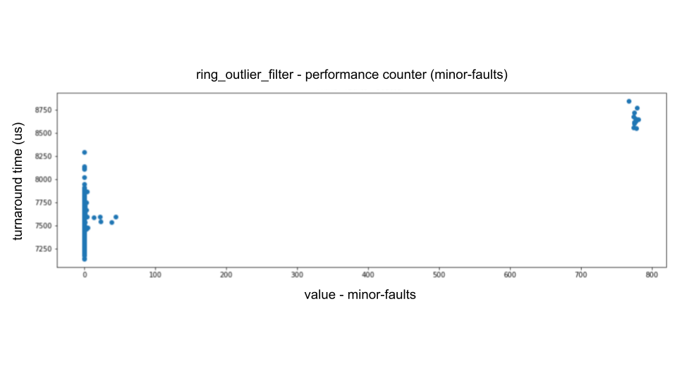
When analyzing the performance of the sensing module from the viewpoint of performance counter, pay attention to instructions, LLC-load-misses, LLC-store-misses, cache-misses, and minor-faults.
Analysis of the performance counter shows that the largest fluctuations come from minor-faults (i.e., soft page faults), the second largest from LLC-store-misses and LLC-load-misses (i.e., cache misses in the last level cache), and the slowest fluctuations come from instructions (i.e., message data size fluctuations).
For example, when we plot minor-faults on the horizontal axis and turnaround time on the vertical axis, we can see the following dominant proportional relationship.
To achieve zero soft page faults, heap allocations must only be made from areas that have been first touched in advance.
We have developed a library called heaphook to avoid soft page faults while running Autoware callback.
If you are interested, refer to the GitHub discussion and the issue.
To reduce LLC misses, it is necessary to reduce the working set and to use cache-efficient access patterns.
In the sensing component, which handles large message data such as LiDAR point cloud data, minimizing copying is important.
A callback that takes sensor data message types as input and output should be written in an in-place algorithm as much as possible.
This means that in the following pseudocode, when generating output_msg from input_msg, it is crucial to avoid using buffers as much as possible to reduce the number of memory copies.
void callback(const PointCloudMsg &input_msg) {
  auto output_msg = allocate_msg<PointCloudMsg>(output_size);
  fill(input_msg, output_msg);
  publish(std::move(output_msg));
}
To improve cache efficiency, implement an in-place style as much as possible, instead of touching memory areas sporadically. In ROS applications using PCL, the code shown below is often seen.
void callback(const sensor_msgs::PointCloud2ConstPtr &input_msg) {
  pcl::PointCloud<PointT>::Ptr input_pcl(new pcl::PointCloud<PointT>);
  pcl::fromROSMsg(*input_msg, *input_pcl);

  // Algorithm is described for point cloud type of pcl
  pcl::PointCloud<PointT>::Ptr output_pcl(new pcl::PointCloud<PointT>);
  fill_pcl(*input_pcl, *output_pcl);

  auto output_msg = allocate_msg<sensor_msgs::PointCloud2>(output_size);
  pcl::toROSMsg(*output_pcl, *output_msg);
  publish(std::move(output_msg));
}
To use the PCL library, fromROSMsg() and toROSMsg() are used to perform message type conversion at the beginning and end of the callback.
This is a wasteful copying process and should be avoided.
We should eliminate unnecessary type conversions by removing dependencies on PCL (e.g., https://github.com/tier4/velodyne_vls/pull/39).
For large message types such as map data, there should be only one instance in the entire system in terms of physical memory.
Planning component#
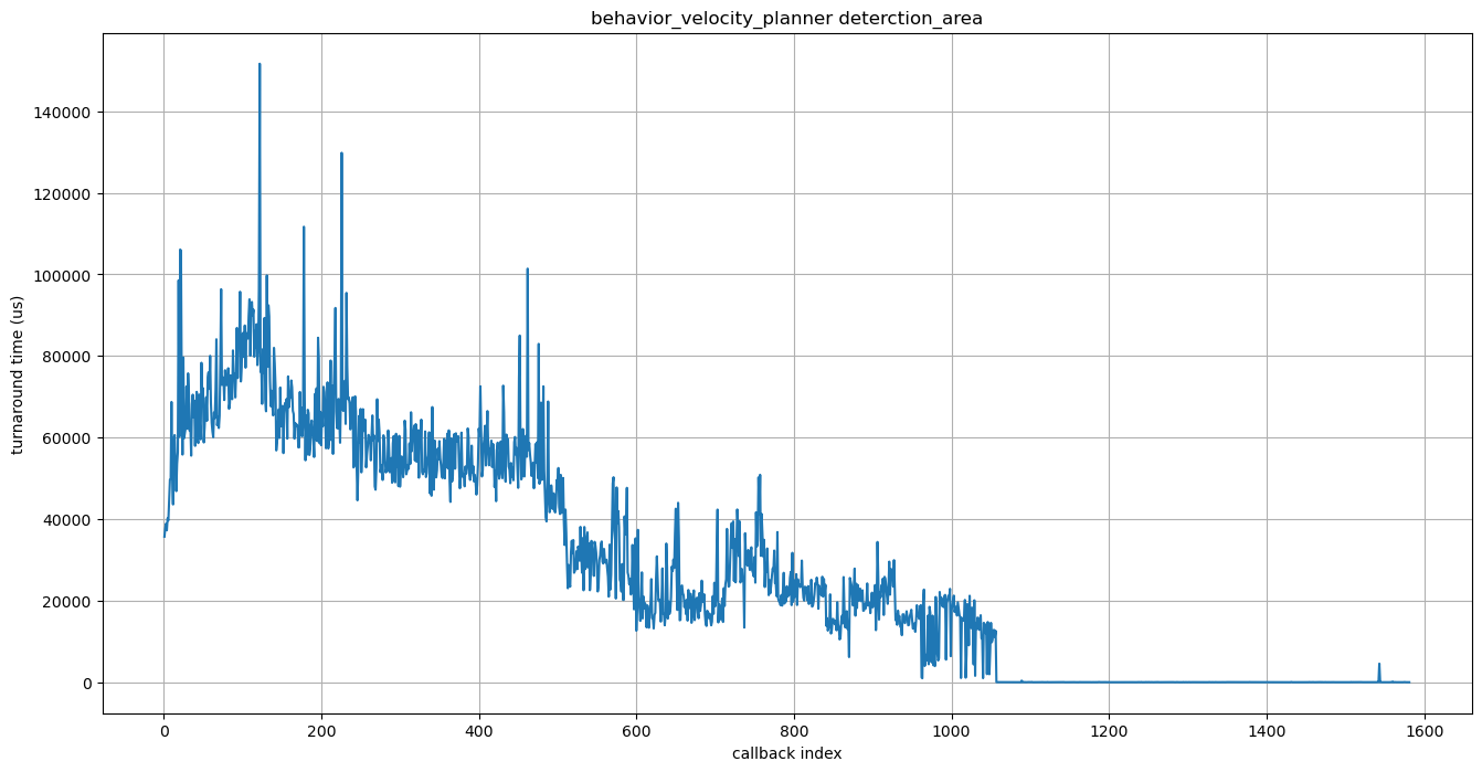
First, we will pick up detection_area module in behavior_velocity_planner node, which tends to have long turnaround time.
We have followed the performance analysis steps above to obtain the following graph.
Axises are the same as the graphs in the sensing case study.
Using pmu_analyzer tool to further identify the bottleneck, we have found that the following multiple loops were taking up a lot of processing time:
for ( area : detection_areas )
  for ( point : point_clouds )
    if ( boost::geometry::within(point, area) )
      // do something with O(1)
It checks whether each point cloud is contained in each detection area.
Let N be the size of point_clouds and M be the size of detection_areas, then the computational complexity of this program is O(N^2 * M), since the complexity of within is O(N). Here, given that most of the point clouds are located far away from a certain detection area, a certain optimization can be achieved. First, calculate the minimum enclosing circle that completely covers the detection area, and then check whether the points are contained in that circle. Most of the point clouds can be quickly ruled out by this method, we don’t have to call the within function in most cases. Below is the pseudocode after optimization.
for ( area : detection_areas )
  circle = calc_minimum_enclosing_circle(area)
  for ( point : point_clouds )
    if ( point is in circle )
      if ( boost::geometry::within(point, area) )
        // do something with O(1)
By using O(N) algorithm for minimum enclosing circle, the computational complexity of this program is reduced to almost O(N * (N + M)) (note that the exact computational complexity does not really change). If you are interested, refer to the Pull Request.
Similar to this example, in the planning component, we take into consideration thousands to tens of thousands of point clouds, thousands of points in a path representing our own route, and polygons representing obstacles and detection areas in the surroundings, and we repeatedly create paths based on them. Therefore, we access the contents of the point clouds and paths multiple times using for-loops. In most cases, the bottleneck lies in these naive for-loops. Here, understanding Big O notation and reducing the order of computational complexity directly leads to performance improvements.