ButterworthFilter
Butterworth Low-pass Filter Design Tool Class#
This Butterworth low-pass filter design tool can be used to design a Butterworth filter in continuous and discrete-time from the given specifications of the filter performance. The Butterworth filter is a class implementation. A default constructor creates the object without any argument.
The filter can be prepared in three ways. If the filter specifications are known, such as the pass-band, and stop-band frequencies (Wp and Ws) together with the pass-band and stop-band ripple magnitudes (Ap and As), one can call the filter's buttord method with these arguments to obtain the recommended filter order (N) and cut-off frequency (Wc_rad_sec [rad/s]).
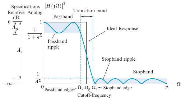 Figure 1. Butterworth Low-pass filter specification from [1].
An example call is demonstrated below;
ButterworthFilter bf();

Wp = 2.0; // pass-band frequency [rad/sec]
Ws = 3.0; // stop-band frequency [rad/sec]
Ap = 6.0; // pass-band ripple mag or loss [dB]
As = 20.0; // stop band ripple attenuation [dB]

// Computing filter coefficients from the specs
bf.Buttord(Wp, Ws, Ap, As);

// Get the computed order and Cut-Off frequency
sOrderCutOff NWc = bf.getOrderCutOff();]

cout << " The computed order is ;" << NWc.N << endl;
cout << " The computed cut-off frequency is ;" << NWc.Wc_rad_sec << endl;
The filter order and cut-off frequency can be obtained in a struct using bf.getOrderCutoff() method. These specs can be printed on the screen by calling PrintFilterSpecs() method. If the user would like to define the order and cut-off frequency manually, the setter methods for these variables can be called to set the filter order (N) and the desired cut-off frequency (Wc_rad_sec [rad/sec]) for the filter.
Obtaining Filter Transfer Functions#
The discrete transfer function of the filter requires the roots and gain of the continuous-time transfer function. Therefore, it is a must to call the first computeContinuousTimeTF() to create the continuous-time transfer function of the filter using;
bf.computeContinuousTimeTF();
The computed continuous-time transfer function roots can be printed on the screen using the methods;
bf.PrintFilter_ContinuousTimeRoots();
bf.PrintContinuousTimeTF();
The resulting screen output for a 5th order filter is demonstrated below.
 Roots of Continuous Time Filter Transfer Function Denominator are :
-0.585518 + j 1.80204
-1.53291 + j 1.11372
-1.89478 + j 2.32043e-16
-1.53291 + j -1.11372
-0.585518 + j -1.80204


The Continuous-Time Transfer Function of the Filter is ;

                                   24.422
-------------------------------------------------------------------------------
1.000 *s[5] + 6.132 *s[4] + 18.798 *s[3] + 35.619 *s[2] + 41.711 *s[1] + 24.422
Discrete Time Transfer Function (Difference Equations)#
The digital filter equivalent of the continuous-time definitions is produced by using the bi-linear transformation. When creating the discrete-time function of the ButterworthFilter object, its Numerator (Bn) and Denominator (An ) coefficients are stored in a vector of filter order size N.
The discrete transfer function method is called using ;
bf.computeDiscreteTimeTF();
bf.PrintDiscreteTimeTF();
The results are printed on the screen like; The Discrete-Time Transfer Function of the Filter is ;
0.191 *z[-5] + 0.956 *z[-4] + 1.913 *z[-3] + 1.913 *z[-2] + 0.956 *z[-1] + 0.191
--------------------------------------------------------------------------------
1.000 *z[-5] + 1.885 *z[-4] + 1.888 *z[-3] + 1.014 *z[-2] + 0.298 *z[-1] + 0.037
and the associated difference coefficients An and Bn by withing a struct ;
sDifferenceAnBn AnBn = bf.getAnBn();
The difference coefficients appear in the filtering equation in the form of.
An * Y_filtered = Bn * Y_unfiltered
To filter a signal given in a vector form ;
Calling Filter by a specified cut-off and sampling frequencies [in Hz]#
The Butterworth filter can also be created by defining the desired order (N), a cut-off frequency (fc in [Hz]), and a sampling frequency (fs in [Hz]). In this method, the cut-off frequency is pre-warped with respect to the sampling frequency [1, 2] to match the continuous and digital filter frequencies.
The filter is prepared by the following calling options;
 // 3rd METHOD defining a sampling frequency together with the cut-off fc, fs
 bf.setOrder(2);
 bf.setCutOffFrequency(10, 100);
At this step, we define a boolean variable whether to use the pre-warping option or not.
// Compute Continuous Time TF
bool use_sampling_frequency = true;
bf.computeContinuousTimeTF(use_sampling_frequency);
bf.PrintFilter_ContinuousTimeRoots();
bf.PrintContinuousTimeTF();

// Compute Discrete Time TF
bf.computeDiscreteTimeTF(use_sampling_frequency);
bf.PrintDiscreteTimeTF();
References:
-
Manolakis, Dimitris G., and Vinay K. Ingle. Applied digital signal processing: theory and practice. Cambridge University Press, 2011.
-
https://en.wikibooks.org/wiki/Digital_Signal_Processing/Bilinear_Transform