Models used in this module#
Tracking model#
CTRV model [1]#
CTRV model is a model that assumes constant turn rate and velocity magnitude.
- state transition equation
- jacobian
Kinematic bicycle model [2]#
Kinematic bicycle model uses slip angle \(\beta\) and velocity \(v\) to calculate yaw update. The merit of using this model is that it can prevent unintended yaw rotation when the vehicle is stopped.
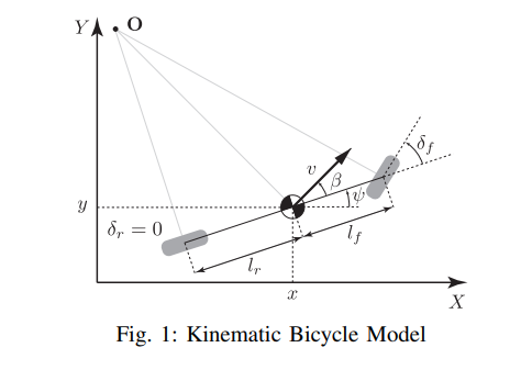
- state variable
- pose( \(x,y\) ), yaw( \(\psi\) ), velocity( \(v\) ), and slip angle ( \(\beta\) )
- \([x_{k}, y_{k}, \psi_{k}, v_{k}, \beta_{k} ]^\mathrm{T}\)
- Prediction Equation
- \(dt\): sampling time
- \(w_{k} = \dot\psi_{k} = \frac{ v_{k} \sin \left( \beta_{k} \right) }{ l_r }\) : angular velocity
- Jacobian
remarks on the output twist#
Remarks that the velocity \(v_{k}\) is the norm of velocity of vehicle, not the longitudinal velocity. So the output twist in the object coordinate \((x,y)\) is calculated as follows.
Anchor point based estimation#
To separate the estimation of the position and the shape, we use anchor point based position estimation.
Anchor point and tracking relationships#
Anchor point is set when the tracking is initialized. Its position is equal to the center of the bounding box of the first tracking bounding box.
Here show how anchor point is used in tracking.

Raw detection is converted to anchor point coordinate, and tracking
Manage anchor point offset#
Anchor point should be kept in the same position of the object. In other words, the offset value must be adjusted so that the input BBOX and the output BBOX's closest plane to the ego vehicle are at the same position.
Known limits, drawbacks#
- When the anchor point is further than the detection center, the tracking will be more affected by the yaw detection noise.
- This can be result in unintended yaw rotation or position drift.
References#
[1] Schubert, Robin & Richter, Eric & Wanielik, Gerd. (2008). Comparison and evaluation of advanced motion models for vehicle tracking. 1 - 6. 10.1109/ICIF.2008.4632283.
[2] Kong, Jason & Pfeiffer, Mark & Schildbach, Georg & Borrelli, Francesco. (2015). Kinematic and dynamic vehicle models for autonomous driving control design. 1094-1099. 10.1109/IVS.2015.7225830.